


Summary
In the following Assignment, we forecast the total cost for two tourists staying four nights in an Airbnb in Istanbul. To carry out this order, we have downloaded the data from insideairbnb.com.
We carried out the following steps to prepare the Data:
First, we imported the data with “vroom”. Then we looked at the data set and determined the variables that were important for us. We also examined the data in detail and decided how we would clean up the data set.
For our second step, we started to cleanse the data. We treated missing data, changed the property to the correct variables (character variables to numeric values).
We also created new variables. For example, we clustered the apartment type, taking the four largest and filtering the rest to “Others” or we counted the minimum nights and filtered for minimum nights less than or equal to four since we determine the price for tourists who only want to stay four nights.
We have also noticed that our data set has many outliers. To get rid of outliers, we have taken out prices above 2000 and equal to 0, because we believe that these prices are unrealistic since there, for example, no places for free
After we cleaned, adjusted and visualised the data, we started modelling with different factors. After variations of models with different factors, we found our model with the best fitted R-square. Then we filtered by our assumptions, such as two bedrooms, one bathroom, located in the city centre, and found our predicted price with a confidence interval of 95%. Our model predicted a price for two people to stay four nights in Istanbul of USD 670.8, with a 95% confidence interval between USD 644.74 and USD 697.92.
Preparing the data - Data wrangling, handling missing values, outliers, etc
We load the data:
listings <- vroom("http://data.insideairbnb.com/turkey/marmara/istanbul/2020-06-28/data/listings.csv.gz")
glimpse(listings)
## Rows: 23,728
## Columns: 106
## $ id <dbl> 4826, 20815, 27271, 2827…
## $ listing_url <chr> "https://www.airbnb.com/…
## $ scrape_id <dbl> 2.02e+13, 2.02e+13, 2.02…
## $ last_scraped <date> 2020-06-28, 2020-06-29,…
## $ name <chr> "The Place", "The Bospho…
## $ summary <chr> "My place is close to gr…
## $ space <chr> "A double bed apartment …
## $ description <chr> "My place is close to gr…
## $ experiences_offered <chr> "none", "none", "none", …
## $ neighborhood_overview <chr> NA, "The lovely neighbor…
## $ notes <chr> NA, "The house may be su…
## $ transit <chr> NA, "The city center, Ta…
## $ access <chr> NA, "Our dear guests may…
## $ interaction <chr> NA, "Depending on our ti…
## $ house_rules <chr> NA, "- Windows facing th…
## $ thumbnail_url <lgl> NA, NA, NA, NA, NA, NA, …
## $ medium_url <lgl> NA, NA, NA, NA, NA, NA, …
## $ picture_url <chr> "https://a0.muscache.com…
## $ xl_picture_url <lgl> NA, NA, NA, NA, NA, NA, …
## $ host_id <dbl> 6603, 78838, 117026, 121…
## $ host_url <chr> "https://www.airbnb.com/…
## $ host_name <chr> "Kaan", "Gülder", "Mutlu…
## $ host_since <date> 2009-01-14, 2010-02-08,…
## $ host_location <chr> "Istanbul, Istanbul, Tur…
## $ host_about <chr> "Hello...\r\nI am Kaan a…
## $ host_response_time <chr> "N/A", "N/A", "N/A", "N/…
## $ host_response_rate <chr> "N/A", "N/A", "N/A", "N/…
## $ host_acceptance_rate <chr> "N/A", "N/A", "50%", "10…
## $ host_is_superhost <lgl> FALSE, FALSE, FALSE, FAL…
## $ host_thumbnail_url <chr> "https://a0.muscache.com…
## $ host_picture_url <chr> "https://a0.muscache.com…
## $ host_neighbourhood <chr> "Üsküdar", "Beşiktaş", "…
## $ host_listings_count <dbl> 1, 2, 1, 20, 1, 1, 1, 2,…
## $ host_total_listings_count <dbl> 1, 2, 1, 20, 1, 1, 1, 2,…
## $ host_verifications <chr> "['email', 'phone', 'fac…
## $ host_has_profile_pic <lgl> TRUE, TRUE, TRUE, TRUE, …
## $ host_identity_verified <lgl> FALSE, FALSE, TRUE, FALS…
## $ street <chr> "Istanbul Province, Ista…
## $ neighbourhood <chr> "Üsküdar", "Beşiktaş", "…
## $ neighbourhood_cleansed <chr> "Uskudar", "Besiktas", "…
## $ neighbourhood_group_cleansed <lgl> NA, NA, NA, NA, NA, NA, …
## $ city <chr> "Istanbul Province", "Is…
## $ state <chr> "Istanbul", NA, NA, NA, …
## $ zipcode <chr> "34684", "34345", "34433…
## $ market <chr> "Istanbul", "Istanbul", …
## $ smart_location <chr> "Istanbul Province, Turk…
## $ country_code <chr> "TR", "TR", "TR", "TR", …
## $ country <chr> "Turkey", "Turkey", "Tur…
## $ latitude <dbl> 41.1, 41.1, 41.0, 41.0, …
## $ longitude <dbl> 29.1, 29.0, 29.0, 29.0, …
## $ is_location_exact <lgl> FALSE, TRUE, FALSE, TRUE…
## $ property_type <chr> "Apartment", "Apartment"…
## $ room_type <chr> "Entire home/apt", "Enti…
## $ accommodates <dbl> 2, 3, 2, 5, 2, 3, 2, 2, …
## $ bathrooms <dbl> 1.0, 1.0, 1.0, 1.0, 1.0,…
## $ bedrooms <dbl> 0, 2, 1, 1, 2, 1, 1, 1, …
## $ beds <dbl> 1, 2, 1, 3, 2, 1, 1, 1, …
## $ bed_type <chr> "Real Bed", "Real Bed", …
## $ amenities <chr> "{TV,\"Cable TV\",Intern…
## $ square_feet <dbl> 700, NA, NA, 753, 700, 0…
## $ price <chr> "$720.00", "$816.00", "$…
## $ weekly_price <chr> NA, "$1,556.00", "$1,769…
## $ monthly_price <chr> NA, "$5,327.00", "$6,307…
## $ security_deposit <chr> NA, "$679.00", "$769.00"…
## $ cleaning_fee <chr> NA, NA, "$308.00", "$77.…
## $ guests_included <dbl> 2, 4, 2, 2, 6, 1, 1, 2, …
## $ extra_people <chr> "$178.00", "$240.00", "$…
## $ minimum_nights <dbl> 1, 365, 30, 3, 3, 3, 1, …
## $ maximum_nights <dbl> 730, 900, 90, 360, 60, 1…
## $ minimum_minimum_nights <dbl> 1, 365, 30, 3, 3, 3, 1, …
## $ maximum_minimum_nights <dbl> 1, 365, 30, 3, 3, 3, 1, …
## $ minimum_maximum_nights <dbl> 730, 900, 90, 360, 60, 1…
## $ maximum_maximum_nights <dbl> 730, 900, 90, 360, 60, 1…
## $ minimum_nights_avg_ntm <dbl> 1, 365, 30, 3, 3, 3, 1, …
## $ maximum_nights_avg_ntm <dbl> 730, 900, 90, 360, 60, 1…
## $ calendar_updated <chr> "38 months ago", "7 mont…
## $ has_availability <lgl> TRUE, TRUE, TRUE, TRUE, …
## $ availability_30 <dbl> 30, 13, 28, 30, 28, 29, …
## $ availability_60 <dbl> 60, 26, 58, 60, 58, 59, …
## $ availability_90 <dbl> 90, 36, 80, 90, 88, 89, …
## $ availability_365 <dbl> 365, 279, 289, 365, 88, …
## $ calendar_last_scraped <date> 2020-06-28, 2020-06-29,…
## $ number_of_reviews <dbl> 1, 41, 13, 0, 0, 0, 1, 1…
## $ number_of_reviews_ltm <dbl> 0, 0, 0, 0, 0, 0, 0, 0, …
## $ first_review <date> 2009-06-01, 2010-03-24,…
## $ last_review <date> 2009-06-01, 2018-11-07,…
## $ review_scores_rating <dbl> 100, 90, 98, NA, NA, NA,…
## $ review_scores_accuracy <dbl> NA, 9, 10, NA, NA, NA, N…
## $ review_scores_cleanliness <dbl> NA, 9, 9, NA, NA, NA, NA…
## $ review_scores_checkin <dbl> NA, 10, 10, NA, NA, NA, …
## $ review_scores_communication <dbl> NA, 10, 10, NA, NA, NA, …
## $ review_scores_location <dbl> NA, 10, 10, NA, NA, NA, …
## $ review_scores_value <dbl> NA, 9, 10, NA, NA, NA, N…
## $ requires_license <lgl> FALSE, FALSE, FALSE, FAL…
## $ license <lgl> NA, NA, NA, NA, NA, NA, …
## $ jurisdiction_names <lgl> NA, NA, NA, NA, NA, NA, …
## $ instant_bookable <lgl> FALSE, FALSE, FALSE, TRU…
## $ is_business_travel_ready <lgl> FALSE, FALSE, FALSE, FAL…
## $ cancellation_policy <chr> "flexible", "moderate", …
## $ require_guest_profile_picture <lgl> FALSE, TRUE, FALSE, FALS…
## $ require_guest_phone_verification <lgl> FALSE, FALSE, FALSE, FAL…
## $ calculated_host_listings_count <dbl> 1, 2, 1, 19, 1, 1, 1, 2,…
## $ calculated_host_listings_count_entire_homes <dbl> 1, 1, 1, 6, 1, 0, 0, 1, …
## $ calculated_host_listings_count_private_rooms <dbl> 0, 1, 0, 0, 0, 1, 1, 1, …
## $ calculated_host_listings_count_shared_rooms <dbl> 0, 0, 0, 0, 0, 0, 0, 0, …
## $ reviews_per_month <dbl> 0.01, 0.33, 0.19, NA, NA…We can rapidly see our listings data frame using glimpse() function. Below is a description of the most important variables for this project:
price: cost per night
cleaning_fee: cleaning fee
extra_people: charge for having more than 1 person
property_type: type of accommodation (House, Apartment, etc.)
room_type:
- Entire home/apt (guests have entire place to themselves)
- Private room (Guests have private room to sleep, all other rooms shared)
- Shared room (Guests sleep in room shared with others)
number_of_reviews: Total number of reviews for the listing
review_scores_rating: Average review score (0 - 100)
longitude, latitude: geographical coordinates to help us locate the listing
neighbourhood: three variables on a few major neighbourhoods
The first step is to prepare the data for our work, by modifying the variables that need so.
With the glimpse() function before, we have seen that price, cleaning_fee and extra_people is a character variable, but it would be more useful and logical for them to be numeric (double). We transform those variables with the following code.
listing <- listings %>%
  mutate(price = parse_number(price)) %>%
  mutate(weekly_price = parse_number(weekly_price)) %>%
  mutate(monthly_price = parse_number(monthly_price)) %>%
  mutate(security_deposit = parse_number(security_deposit)) %>%
  mutate(cleaning_fee = parse_number(cleaning_fee)) %>%
  mutate(extra_people = parse_number(extra_people))

#With typeof() we check that the type of variable has changed correctly to double
typeof(listing$price)
## [1] "double"typeof(listing$weekly_price)## [1] "double"typeof(listing$monthly_price)## [1] "double"typeof(listing$security_deposit)## [1] "double"typeof(listing$cleaning_fee)## [1] "double"typeof(listing$extra_people)## [1] "double"We skim() through the data set to get some more information. For example, for every data set it is worth checking if there is something weird regarding missing values, such as important variables having a lot of (or all) missing values.
skim(listing)| Name | listing |
| Number of rows | 23728 |
| Number of columns | 106 |
| _______________________ | |
| Column type frequency: | |
| character | 40 |
| Date | 5 |
| logical | 16 |
| numeric | 45 |
| ________________________ | |
| Group variables | None |
Variable type: character
| skim_variable | n_missing | complete_rate | min | max | empty | n_unique | whitespace |
|---|---|---|---|---|---|---|---|
| listing_url | 0 | 1.00 | 33 | 37 | 0 | 23728 | 0 |
| name | 54 | 1.00 | 1 | 108 | 0 | 22685 | 0 |
| summary | 3779 | 0.84 | 1 | 1000 | 0 | 17202 | 1 |
| space | 11361 | 0.52 | 1 | 1000 | 0 | 10575 | 0 |
| description | 2876 | 0.88 | 1 | 1000 | 0 | 18952 | 0 |
| experiences_offered | 0 | 1.00 | 4 | 4 | 0 | 1 | 0 |
| neighborhood_overview | 12658 | 0.47 | 1 | 1000 | 0 | 8867 | 0 |
| notes | 18474 | 0.22 | 1 | 1000 | 0 | 4221 | 0 |
| transit | 13660 | 0.42 | 1 | 1000 | 0 | 8147 | 0 |
| access | 16337 | 0.31 | 1 | 1000 | 0 | 5943 | 0 |
| interaction | 15019 | 0.37 | 1 | 1000 | 0 | 6607 | 0 |
| house_rules | 16407 | 0.31 | 1 | 1000 | 0 | 6306 | 0 |
| picture_url | 0 | 1.00 | 80 | 146 | 0 | 22996 | 0 |
| host_url | 0 | 1.00 | 38 | 43 | 0 | 14450 | 0 |
| host_name | 1 | 1.00 | 1 | 35 | 0 | 4907 | 0 |
| host_location | 83 | 1.00 | 2 | 105 | 0 | 775 | 0 |
| host_about | 11902 | 0.50 | 1 | 5717 | 0 | 6144 | 10 |
| host_response_time | 1 | 1.00 | 3 | 18 | 0 | 5 | 0 |
| host_response_rate | 1 | 1.00 | 2 | 4 | 0 | 60 | 0 |
| host_acceptance_rate | 1 | 1.00 | 2 | 4 | 0 | 85 | 0 |
| host_thumbnail_url | 1 | 1.00 | 55 | 106 | 0 | 14358 | 0 |
| host_picture_url | 1 | 1.00 | 57 | 109 | 0 | 14358 | 0 |
| host_neighbourhood | 15027 | 0.37 | 4 | 33 | 0 | 59 | 0 |
| host_verifications | 0 | 1.00 | 2 | 158 | 0 | 277 | 0 |
| street | 0 | 1.00 | 10 | 116 | 0 | 1180 | 0 |
| neighbourhood | 5377 | 0.77 | 4 | 15 | 0 | 15 | 0 |
| neighbourhood_cleansed | 0 | 1.00 | 4 | 13 | 0 | 39 | 0 |
| city | 773 | 0.97 | 2 | 69 | 0 | 641 | 0 |
| state | 397 | 0.98 | 1 | 58 | 0 | 293 | 0 |
| zipcode | 2422 | 0.90 | 1 | 43 | 0 | 388 | 0 |
| market | 0 | 1.00 | 7 | 21 | 0 | 3 | 0 |
| smart_location | 0 | 1.00 | 6 | 77 | 0 | 706 | 0 |
| country_code | 0 | 1.00 | 2 | 2 | 0 | 3 | 0 |
| country | 0 | 1.00 | 6 | 12 | 0 | 3 | 0 |
| property_type | 0 | 1.00 | 3 | 22 | 0 | 43 | 0 |
| room_type | 0 | 1.00 | 10 | 15 | 0 | 4 | 0 |
| bed_type | 0 | 1.00 | 5 | 13 | 0 | 5 | 0 |
| amenities | 0 | 1.00 | 2 | 1297 | 0 | 21255 | 0 |
| calendar_updated | 0 | 1.00 | 5 | 14 | 0 | 104 | 0 |
| cancellation_policy | 0 | 1.00 | 6 | 27 | 0 | 6 | 0 |
Variable type: Date
| skim_variable | n_missing | complete_rate | min | max | median | n_unique |
|---|---|---|---|---|---|---|
| last_scraped | 0 | 1.00 | 2020-06-28 | 2020-06-30 | 2020-06-29 | 3 |
| host_since | 1 | 1.00 | 2009-01-14 | 2020-06-27 | 2017-08-27 | 3095 |
| calendar_last_scraped | 0 | 1.00 | 2020-06-28 | 2020-06-30 | 2020-06-29 | 3 |
| first_review | 12375 | 0.48 | 2009-06-01 | 2020-06-29 | 2019-04-12 | 2216 |
| last_review | 12375 | 0.48 | 2009-06-01 | 2020-06-29 | 2020-01-01 | 1424 |
Variable type: logical
| skim_variable | n_missing | complete_rate | mean | count |
|---|---|---|---|---|
| thumbnail_url | 23728 | 0 | NaN | : |
| medium_url | 23728 | 0 | NaN | : |
| xl_picture_url | 23728 | 0 | NaN | : |
| host_is_superhost | 1 | 1 | 0.11 | FAL: 21147, TRU: 2580 |
| host_has_profile_pic | 1 | 1 | 1.00 | TRU: 23625, FAL: 102 |
| host_identity_verified | 1 | 1 | 0.16 | FAL: 19951, TRU: 3776 |
| neighbourhood_group_cleansed | 23728 | 0 | NaN | : |
| is_location_exact | 0 | 1 | 0.35 | FAL: 15329, TRU: 8399 |
| has_availability | 0 | 1 | 1.00 | TRU: 23728 |
| requires_license | 0 | 1 | 0.00 | FAL: 23728 |
| license | 23728 | 0 | NaN | : |
| jurisdiction_names | 23728 | 0 | NaN | : |
| instant_bookable | 0 | 1 | 0.60 | TRU: 14249, FAL: 9479 |
| is_business_travel_ready | 0 | 1 | 0.00 | FAL: 23728 |
| require_guest_profile_picture | 0 | 1 | 0.01 | FAL: 23571, TRU: 157 |
| require_guest_phone_verification | 0 | 1 | 0.01 | FAL: 23526, TRU: 202 |
Variable type: numeric
| skim_variable | n_missing | complete_rate | mean | sd | p0 | p25 | p50 | p75 | p100 | hist |
|---|---|---|---|---|---|---|---|---|---|---|
| id | 0 | 1.00 | 2.91e+07 | 1.31e+07 | 4.83e+03 | 2.10e+07 | 3.40e+07 | 3.97e+07 | 4.40e+07 | ▂▂▂▃▇ |
| scrape_id | 0 | 1.00 | 2.02e+13 | 0.00e+00 | 2.02e+13 | 2.02e+13 | 2.02e+13 | 2.02e+13 | 2.02e+13 | ▁▁▇▁▁ |
| host_id | 0 | 1.00 | 1.49e+08 | 1.16e+08 | 6.60e+03 | 3.29e+07 | 1.48e+08 | 2.59e+08 | 3.52e+08 | ▇▂▃▅▃ |
| host_listings_count | 1 | 1.00 | 2.43e+01 | 2.24e+02 | 0.00e+00 | 1.00e+00 | 1.00e+00 | 4.00e+00 | 3.77e+03 | ▇▁▁▁▁ |
| host_total_listings_count | 1 | 1.00 | 2.43e+01 | 2.24e+02 | 0.00e+00 | 1.00e+00 | 1.00e+00 | 4.00e+00 | 3.77e+03 | ▇▁▁▁▁ |
| latitude | 0 | 1.00 | 4.10e+01 | 5.00e-02 | 4.08e+01 | 4.10e+01 | 4.10e+01 | 4.10e+01 | 4.15e+01 | ▁▇▁▁▁ |
| longitude | 0 | 1.00 | 2.90e+01 | 1.30e-01 | 2.80e+01 | 2.90e+01 | 2.90e+01 | 2.90e+01 | 2.99e+01 | ▁▁▇▁▁ |
| accommodates | 0 | 1.00 | 3.21e+00 | 2.25e+00 | 1.00e+00 | 2.00e+00 | 2.00e+00 | 4.00e+00 | 1.60e+01 | ▇▁▁▁▁ |
| bathrooms | 86 | 1.00 | 1.21e+00 | 1.04e+00 | 0.00e+00 | 1.00e+00 | 1.00e+00 | 1.00e+00 | 5.00e+01 | ▇▁▁▁▁ |
| bedrooms | 173 | 0.99 | 1.39e+00 | 1.44e+00 | 0.00e+00 | 1.00e+00 | 1.00e+00 | 2.00e+00 | 5.00e+01 | ▇▁▁▁▁ |
| beds | 698 | 0.97 | 2.05e+00 | 2.04e+00 | 0.00e+00 | 1.00e+00 | 1.00e+00 | 2.00e+00 | 7.70e+01 | ▇▁▁▁▁ |
| square_feet | 23492 | 0.01 | 6.05e+02 | 1.21e+03 | 0.00e+00 | 7.00e+01 | 5.38e+02 | 8.07e+02 | 1.74e+04 | ▇▁▁▁▁ |
| price | 0 | 1.00 | 4.85e+02 | 1.97e+03 | 0.00e+00 | 1.37e+02 | 2.47e+02 | 4.46e+02 | 7.69e+04 | ▇▁▁▁▁ |
| weekly_price | 21993 | 0.07 | 2.95e+03 | 4.13e+03 | 8.50e+01 | 1.04e+03 | 2.06e+03 | 3.52e+03 | 8.57e+04 | ▇▁▁▁▁ |
| monthly_price | 22031 | 0.07 | 1.02e+04 | 1.32e+04 | 2.06e+02 | 3.46e+03 | 7.31e+03 | 1.27e+04 | 3.26e+05 | ▇▁▁▁▁ |
| security_deposit | 15623 | 0.34 | 7.26e+02 | 2.38e+03 | 0.00e+00 | 0.00e+00 | 0.00e+00 | 7.00e+02 | 3.52e+04 | ▇▁▁▁▁ |
| cleaning_fee | 13660 | 0.42 | 1.27e+02 | 1.78e+02 | 0.00e+00 | 0.00e+00 | 8.00e+01 | 1.92e+02 | 4.57e+03 | ▇▁▁▁▁ |
| guests_included | 0 | 1.00 | 1.40e+00 | 1.09e+00 | 1.00e+00 | 1.00e+00 | 1.00e+00 | 1.00e+00 | 1.60e+01 | ▇▁▁▁▁ |
| extra_people | 0 | 1.00 | 3.01e+01 | 7.53e+01 | 0.00e+00 | 0.00e+00 | 0.00e+00 | 4.00e+01 | 2.06e+03 | ▇▁▁▁▁ |
| minimum_nights | 0 | 1.00 | 4.53e+00 | 2.76e+01 | 1.00e+00 | 1.00e+00 | 1.00e+00 | 3.00e+00 | 1.12e+03 | ▇▁▁▁▁ |
| maximum_nights | 0 | 1.00 | 9.13e+04 | 1.39e+07 | 1.00e+00 | 6.00e+01 | 1.12e+03 | 1.12e+03 | 2.15e+09 | ▇▁▁▁▁ |
| minimum_minimum_nights | 0 | 1.00 | 4.41e+00 | 2.68e+01 | 1.00e+00 | 1.00e+00 | 1.00e+00 | 2.00e+00 | 1.12e+03 | ▇▁▁▁▁ |
| maximum_minimum_nights | 0 | 1.00 | 4.71e+00 | 2.86e+01 | 1.00e+00 | 1.00e+00 | 1.00e+00 | 3.00e+00 | 1.12e+03 | ▇▁▁▁▁ |
| minimum_maximum_nights | 0 | 1.00 | 9.28e+02 | 9.68e+03 | 1.00e+00 | 3.60e+02 | 1.12e+03 | 1.12e+03 | 1.00e+06 | ▇▁▁▁▁ |
| maximum_maximum_nights | 0 | 1.00 | 9.29e+02 | 9.68e+03 | 1.00e+00 | 3.60e+02 | 1.12e+03 | 1.12e+03 | 1.00e+06 | ▇▁▁▁▁ |
| minimum_nights_avg_ntm | 0 | 1.00 | 4.51e+00 | 2.70e+01 | 1.00e+00 | 1.00e+00 | 1.00e+00 | 3.00e+00 | 1.12e+03 | ▇▁▁▁▁ |
| maximum_nights_avg_ntm | 0 | 1.00 | 9.29e+02 | 9.68e+03 | 1.00e+00 | 3.60e+02 | 1.12e+03 | 1.12e+03 | 1.00e+06 | ▇▁▁▁▁ |
| availability_30 | 0 | 1.00 | 2.21e+01 | 1.21e+01 | 0.00e+00 | 1.70e+01 | 2.90e+01 | 3.00e+01 | 3.00e+01 | ▂▁▁▁▇ |
| availability_60 | 0 | 1.00 | 4.53e+01 | 2.38e+01 | 0.00e+00 | 4.10e+01 | 5.90e+01 | 6.00e+01 | 6.00e+01 | ▂▁▁▁▇ |
| availability_90 | 0 | 1.00 | 6.90e+01 | 3.51e+01 | 0.00e+00 | 6.60e+01 | 8.90e+01 | 9.00e+01 | 9.00e+01 | ▂▁▁▁▇ |
| availability_365 | 0 | 1.00 | 2.28e+02 | 1.47e+02 | 0.00e+00 | 8.90e+01 | 3.02e+02 | 3.65e+02 | 3.65e+02 | ▃▂▂▁▇ |
| number_of_reviews | 0 | 1.00 | 7.87e+00 | 2.32e+01 | 0.00e+00 | 0.00e+00 | 0.00e+00 | 4.00e+00 | 3.45e+02 | ▇▁▁▁▁ |
| number_of_reviews_ltm | 0 | 1.00 | 3.04e+00 | 7.47e+00 | 0.00e+00 | 0.00e+00 | 0.00e+00 | 2.00e+00 | 1.08e+02 | ▇▁▁▁▁ |
| review_scores_rating | 12978 | 0.45 | 9.13e+01 | 1.40e+01 | 2.00e+01 | 9.00e+01 | 9.60e+01 | 1.00e+02 | 1.00e+02 | ▁▁▁▁▇ |
| review_scores_accuracy | 12991 | 0.45 | 9.29e+00 | 1.42e+00 | 2.00e+00 | 9.00e+00 | 1.00e+01 | 1.00e+01 | 1.00e+01 | ▁▁▁▁▇ |
| review_scores_cleanliness | 12988 | 0.45 | 9.06e+00 | 1.51e+00 | 2.00e+00 | 9.00e+00 | 1.00e+01 | 1.00e+01 | 1.00e+01 | ▁▁▁▂▇ |
| review_scores_checkin | 12991 | 0.45 | 9.52e+00 | 1.28e+00 | 2.00e+00 | 1.00e+01 | 1.00e+01 | 1.00e+01 | 1.00e+01 | ▁▁▁▁▇ |
| review_scores_communication | 12987 | 0.45 | 9.55e+00 | 1.24e+00 | 2.00e+00 | 1.00e+01 | 1.00e+01 | 1.00e+01 | 1.00e+01 | ▁▁▁▁▇ |
| review_scores_location | 12991 | 0.45 | 9.44e+00 | 1.23e+00 | 2.00e+00 | 9.00e+00 | 1.00e+01 | 1.00e+01 | 1.00e+01 | ▁▁▁▁▇ |
| review_scores_value | 12993 | 0.45 | 9.19e+00 | 1.40e+00 | 2.00e+00 | 9.00e+00 | 1.00e+01 | 1.00e+01 | 1.00e+01 | ▁▁▁▁▇ |
| calculated_host_listings_count | 0 | 1.00 | 5.86e+00 | 1.65e+01 | 1.00e+00 | 1.00e+00 | 2.00e+00 | 5.00e+00 | 1.76e+02 | ▇▁▁▁▁ |
| calculated_host_listings_count_entire_homes | 0 | 1.00 | 2.81e+00 | 6.37e+00 | 0.00e+00 | 0.00e+00 | 1.00e+00 | 2.00e+00 | 6.60e+01 | ▇▁▁▁▁ |
| calculated_host_listings_count_private_rooms | 0 | 1.00 | 2.46e+00 | 1.51e+01 | 0.00e+00 | 0.00e+00 | 1.00e+00 | 1.00e+00 | 1.75e+02 | ▇▁▁▁▁ |
| calculated_host_listings_count_shared_rooms | 0 | 1.00 | 9.00e-02 | 6.00e-01 | 0.00e+00 | 0.00e+00 | 0.00e+00 | 0.00e+00 | 1.10e+01 | ▇▁▁▁▁ |
| reviews_per_month | 12375 | 0.48 | 7.10e-01 | 9.00e-01 | 1.00e-02 | 1.30e-01 | 3.30e-01 | 9.50e-01 | 9.20e+00 | ▇▁▁▁▁ |
It calls our attention that there are 13600 missing values for cleaning_fee. However, this is an example of data that is missing not at random, since there is a specific pattern/explanation: quite probably, the cleaning fee for those properties is $0 and thus a missing value is actually a 0. We add this modification below.
listing <- listing %>%
  mutate(cleaning_fee = case_when(
    is.na(cleaning_fee) ~ 0,
    TRUE ~ cleaning_fee
  ))
Now, let’s examine property_type, as it is an important variable to describe the general characteristics one should expect from the property. We can use the count() function to determine how many categories are there and their frequency.
#List of the type of properties and their frequency:
listing_type <- listing %>%
  count(property_type) %>%
  arrange(desc(n)) %>%
  mutate(share = n / sum(n), share=scales::percent(share))
listing_type
## # A tibble: 43 x 3
## property_type n share
## <chr> <int> <chr>
## 1 Apartment 14958 63.0394%
## 2 Serviced apartment 1700 7.1645%
## 3 House 1564 6.5914%
## 4 Boutique hotel 1113 4.6907%
## 5 Townhouse 692 2.9164%
## 6 Condominium 629 2.6509%
## 7 Aparthotel 590 2.4865%
## 8 Bed and breakfast 585 2.4654%
## 9 Hotel 545 2.2969%
## 10 Loft 436 1.8375%
## # … with 33 more rows#Top 4 categories represent the vast majority of properties.
#Calculate this percentage:
listing_type_sum <- listing_type %>%
summarise(share = n / sum(n)) %>%
head(4) %>%
summarise(sum = sum(share))
listing_type_sum## # A tibble: 1 x 1
## sum
## <dbl>
## 1 0.815We see that the four most common property types are Apartment, Serviced apartment, House, and Boutique hotel; with 81.5% of properties being represented by these four categories.
Since the vast majority of the observations in the data are one of the top four or five property types, we would like to create a simplified version of property_type variable that has 5 categories: the top four categories and Other.
listing <- listing %>%
  mutate(prop_type_simplified = case_when(
    property_type %in% c("Apartment","Serviced apartment", "House","Boutique hotel") ~ property_type,
    TRUE ~ "Other"
  ))

#Check that prop_type_simplified was correctly made:
listing_prop_sum <- listing %>%
  count(property_type, prop_type_simplified) %>%
  arrange(desc(n))
listing_prop_sum
## # A tibble: 43 x 3
## property_type prop_type_simplified n
## <chr> <chr> <int>
## 1 Apartment Apartment 14958
## 2 Serviced apartment Serviced apartment 1700
## 3 House House 1564
## 4 Boutique hotel Boutique hotel 1113
## 5 Townhouse Other 692
## 6 Condominium Other 629
## 7 Aparthotel Other 590
## 8 Bed and breakfast Other 585
## 9 Hotel Other 545
## 10 Loft Other 436
## # … with 33 more rowsAirbnb is most commonly used for travel purposes, i.e., as an alternative to traditional hotels. We only want to include listings in our regression analysis that are intended for travel purposes.
Thus, our last step in preparing the data for analysis will be to study minimum_nights variable in order to define the most common values and how they are related to the different purposes of Airbnb listings. Remember, we want to exclude other purposes different than traveling, such as short-term rentals for work, etc.
#We check the different values for minimum_nights and their frequency:
listing_nights <- listing %>%
  count(minimum_nights) %>%
  arrange(desc(n))
listing_nights
## # A tibble: 65 x 2
## minimum_nights n
## <dbl> <int>
## 1 1 13228
## 2 2 4511
## 3 3 2682
## 4 7 702
## 5 5 701
## 6 4 490
## 7 30 324
## 8 10 185
## 9 15 179
## 10 6 138
## # … with 55 more rowsWe see that the most common value for minimum_nights is 1, following by 2 and 3. These values look like what we would expect from any property listed for tourists. However, 7 and 30 are also relatively common minimum night requirements, reflecting one week and one month stays, respectively. These are reflections of common time intervals that hosts would like to rent their properties for, likely not for tourism purposes, at least not for the average stay for travelers. These hosts could be looking for less turnover on their properties over longer periods of time by having fewer independent guests, targeting a different market from tourism, such as short-term rents for business purposes or newcomers to Istanbul.
Hence, those properties which are not destined for tourists should be out of the scope of our analysis. For that, we will filter out all properties with a minimum stay of more than 4 nights.
listing <- listing %>%
  filter(minimum_nights <= 4)
Dealing with outliers
Additionally, before starting to build models we should explore if there are outliers that could affect them. We want to build predictive models using data of normal properties, discarding especial situations such as staying at a palace for a price 100 times higher than the average hotel. We can use histograms to check those possible outliers in price.
ggplot(listing, mapping = aes(x = price)) +
  geom_histogram() +
  scale_x_continuous() +
  labs(title = "Distribution of price",
       y = "Number of properties") +
  theme_bw()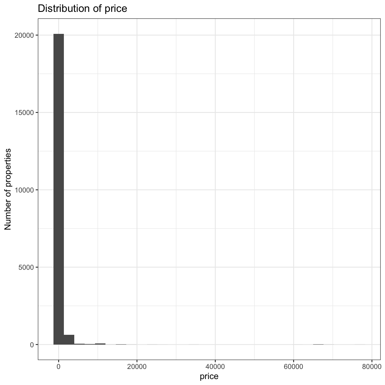
We can see extreme outliers in the price variable. As we said before, we are not interested in these extreme cases for our predictive model, as these can be properties with very special characteristics, very luxurious, or with an absurd price because the host does not want to acomodate hosts at that moment. We will filter out the values above 5000, and run the plot again.
listing_clean <- listing %>%
  filter(price<5000)

ggplot(listing_clean, mapping = aes(x = price)) +
  geom_histogram() +
  scale_x_continuous() +
  labs(title = "Distribution of price",
       y = "Number of properties") +
  theme_bw()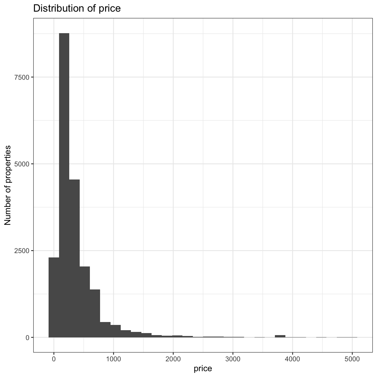
We still see a very fat tail in the last histogram, so we will make one last correction, filtering out outliers with a price greater that 2000, and also discarding the properties with a price of 0, as a property for free does not make sense.
#We will also filter out, just in case, values with a price of 0.
listing_clean <- listing %>%
  filter(price<2000, price>0)

ggplot(listing_clean, mapping = aes(y = reorder(prop_type_simplified, price, median), x = price)) +
  geom_boxplot() +
  scale_x_continuous() +
  labs(title = "Distribution of price and outliers",
       y = "Type of property") +
  theme_bw()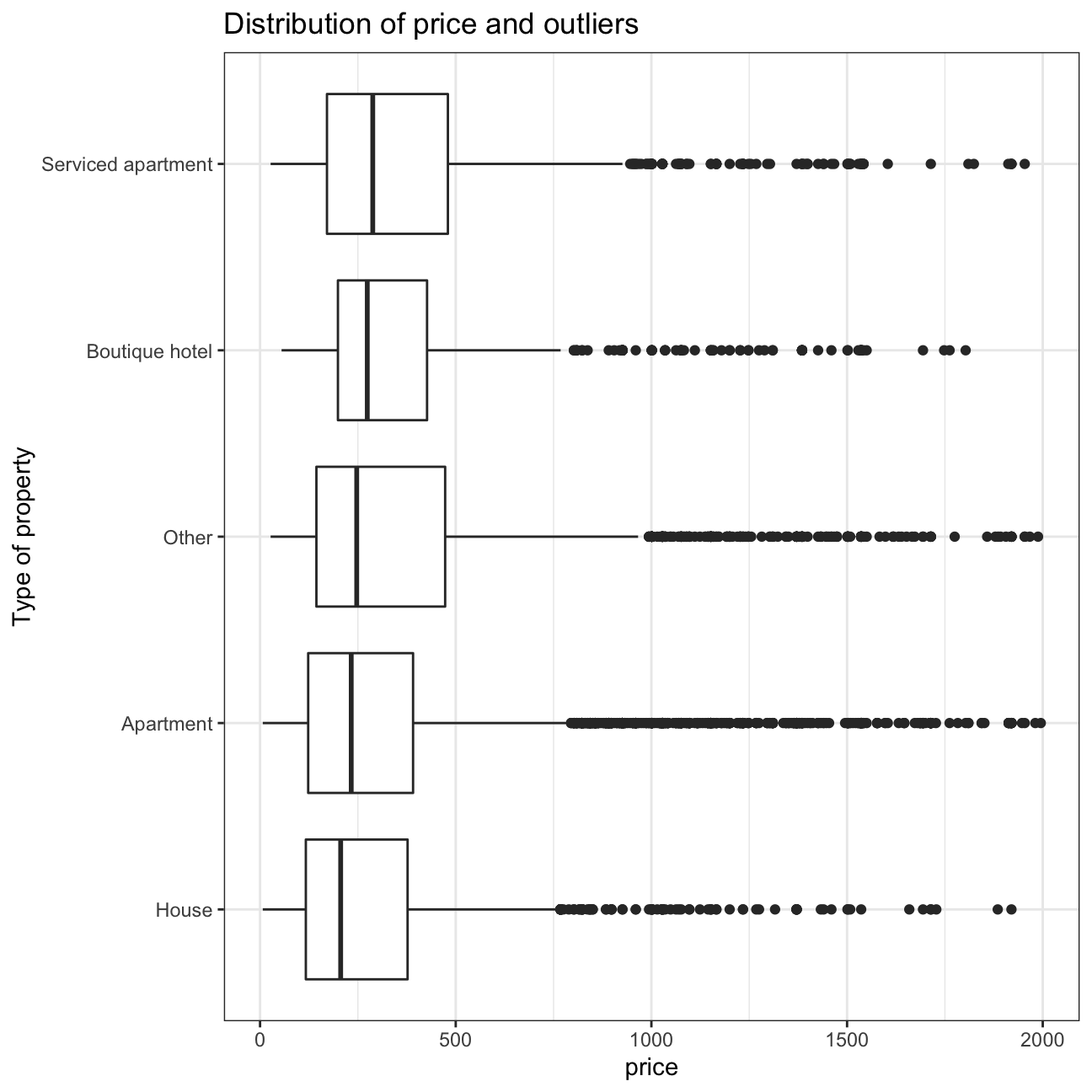
After dealing with the outliers, the data set is ready for our analysis.
Mapping
Visualisations of feature distributions and their relations are key to understanding a data set, and they can open up new lines of exploration. While it is not the main objective of this project to go into geospatial visualisations with R, we will make a map of Istanbul, and overlay all AirBnB coordinates to get an overview of the spatial distribution of AirBnB rentals. For this visualisation we use the leaflet package, which includes a variety of tools for interactive maps, so we can easily zoom in-out, click on a point to get the actual AirBnB listing for that specific point, etc.
The following code, having created a dataframe listings with all AirbnB listings in Bordeaux, will plot on the map all AirBnBs where minimum_nights is less than equal to four (4).
leaflet(data = filter(listing, minimum_nights <= 4)) %>%
  addProviderTiles("OpenStreetMap.Mapnik") %>%
  addCircleMarkers(lng = ~longitude,
                   lat = ~latitude,
                   radius = 1,
                   fillColor = "blue",
                   fillOpacity = 0.4,
                   popup = ~listing_url,
                   label = ~property_type)
Regression analysis
This is the core of this project. We are going develop a regression model to predict the cost for two guests for staying 4 nights in the city.
For the target variable “y”, we will use the cost for two people to stay at an Airbnb location for four (4) nights. For this, we create a new variable called price_4_nights that uses price, cleaning_fee, guests_included, and extra_people to calculate the total cost for two people to stay at the Airbnb property for 4 nights. This is the variable “y” we want to explain.
Now, we will use an histogram to examine the distributions of price_4_nights.
listing_price <- listing_clean %>%
  mutate(price_4_nights = (price * 4) + cleaning_fee + (if_else(guests_included < 2, extra_people, 0)))

ggplot(listing_price, aes(x = price_4_nights)) +
        geom_histogram() +
        labs(title = "Distribution of variable price_4_nights")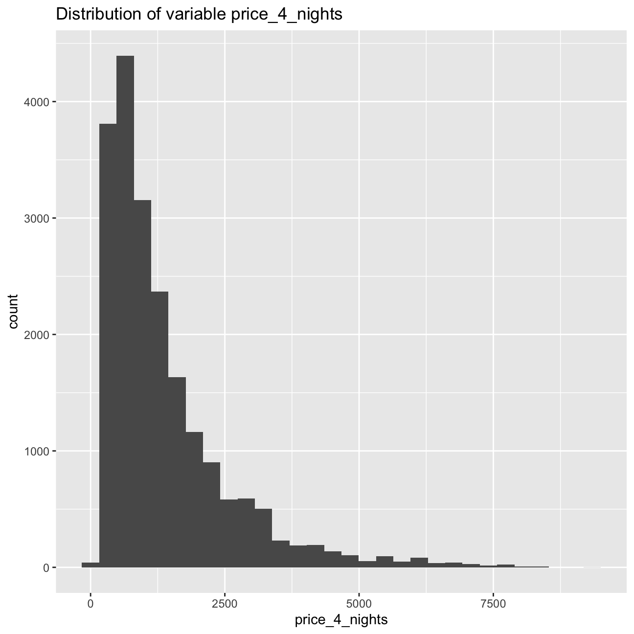
As the data is clearly right-skewed, we should use log(price_4_nights) for our regression model, as a majority of the values are clustered at the low end of the scale. This means that the high price listings create a positively skewed distribution that is difficult to interpret without a logarithmic scale.
#Create log(price_4_nights)
listing_price <- listing_price %>%
  mutate(log_price_4_nights = log(price_4_nights))
#Plot histogram with price_4_nights in logarithmic scale
ggplot(listing_price, aes(x = log_price_4_nights)) +
geom_histogram() +
labs(title = "Distribution of variable ln(price_4_nights)")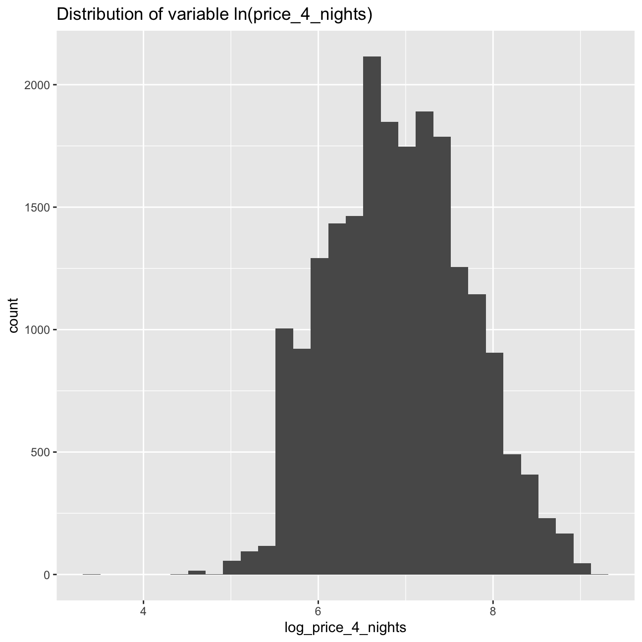
Following, we will use ggpairs to produce a correlation scatterplot with selected numerical variables from the dataset.
#using ggpairs to explore the relationship between some numeric variables of interest
listing_price %>%
  select(log_price_4_nights, number_of_reviews, review_scores_rating, reviews_per_month, bathrooms, bedrooms, beds, accommodates) %>%
  ggpairs(aes(alpha=0.1))+
  theme_bw()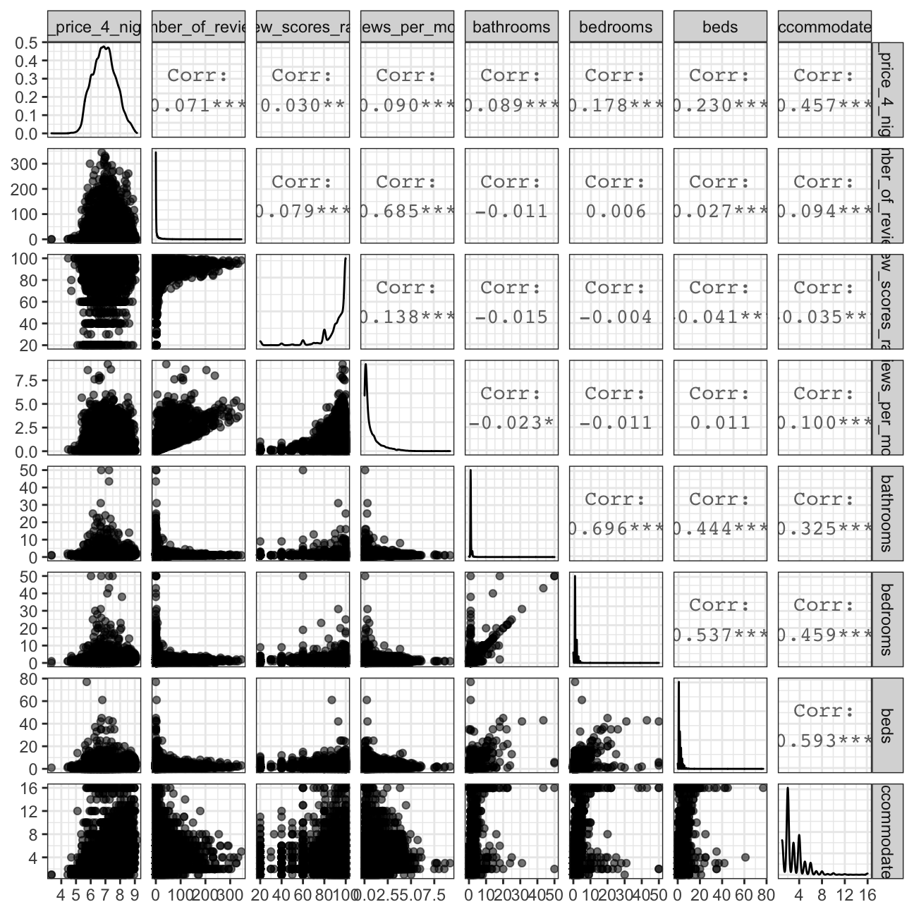
As we see in the scatterplot, there is not very high correlation between log_price_4_nights and the other numerical variables, but they are still significant so we are going to test these variables in our model.
In the next step, we fit a regression model called model1 with the following explanatory variables: prop_type_simplified, number_of_reviews, and review_scores_rating.
We will also use the package broom::“tidy models”, with:
* tidy() for model coefficients
* glance() for model fit
model1 <- lm(log_price_4_nights ~ prop_type_simplified +
                                    number_of_reviews +
                                    review_scores_rating,
             data = listing_price)

model1 %>% broom::tidy(conf.int = TRUE)
## # A tibble: 7 x 7
## term estimate std.error statistic p.value conf.low conf.high
## <chr> <dbl> <dbl> <dbl> <dbl> <dbl> <dbl>
## 1 (Intercept) 6.79 0.0501 136. 0. 6.69e+0 6.89
## 2 prop_type_simplified… 0.00960 0.0332 0.289 7.72e- 1 -5.55e-2 0.0747
## 3 prop_type_simplified… -0.0518 0.0326 -1.59 1.11e- 1 -1.16e-1 0.0120
## 4 prop_type_simplified… -0.00479 0.0212 -0.226 8.21e- 1 -4.63e-2 0.0367
## 5 prop_type_simplified… 0.192 0.0283 6.78 1.25e-11 1.36e-1 0.247
## 6 number_of_reviews 0.00198 0.000225 8.77 2.02e-18 1.53e-3 0.00242
## 7 review_scores_rating 0.00135 0.000534 2.53 1.14e- 2 3.04e-4 0.00240model1 %>% broom::glance()## # A tibble: 1 x 12
## r.squared adj.r.squared sigma statistic p.value df logLik AIC BIC
## <dbl> <dbl> <dbl> <dbl> <dbl> <dbl> <dbl> <dbl> <dbl>
## 1 0.0141 0.0135 0.721 22.7 1.09e-26 6 -10393. 20802. 20860.
## # … with 3 more variables: deviance <dbl>, df.residual <int>, nobs <int>As we obtained an adjusted R-squared value of 0.0135 in model1, we will assess if there are more significant variables to add to our model. Also, we can confirm our choice of log(price_4_nights) against price_4_nights as target variable by running the model with the latter, which gave a lower R-squared value, 0.0084 —that is, “worse” in terms of predictive power.
First, we look at the coefficient of review_scores_rating in terms of price_4_nights. It is negatively correlated with price, and this can happen because guests may be more willing to give higher ratings for properties that did not cost them a lot. Similarly, those paying for more expensive properties probably expect more from their stay and are more likely to give unflattering reviews for minor inconveniences.
Then, looking at the Property type (variable prop_type_simplified), we know that it is a categorical variable, so the coefficients for each of the property types is a reflection of the expected pricing discrepancy between the average apartment, which is the baseline, and the average Boutique hotel, House, etc. Because apartments represent the most basic offering on Airbnb, it makes sense that other, less common listings like boutique hotels and serviced apartments would command a higher price. The negative coefficient on houses is likely more a function of location, as houses in a major city like Istanbul would likely be much further from the city center than apartments.
We would also like to determine if room_type is a significant predictor of the cost for 4 nights, given everything else in the model. For that, we fit another regression model called model2 that includes all of the explanantory variables in model1 plus room_type.
model2 <- lm(log_price_4_nights ~ prop_type_simplified + number_of_reviews + review_scores_rating + room_type, data = listing_price)
model2 %>% broom::tidy(conf.int = TRUE)
## # A tibble: 10 x 7
## term estimate std.error statistic p.value conf.low conf.high
## <chr> <dbl> <dbl> <dbl> <dbl> <dbl> <dbl>
## 1 (Intercept) 7.03e+0 0.0424 166. 0. 6.95e+0 7.11
## 2 prop_type_simplifi… 3.92e-1 0.0313 12.5 1.05e- 35 3.31e-1 0.454
## 3 prop_type_simplifi… 1.74e-2 0.0274 0.633 5.27e- 1 -3.64e-2 0.0711
## 4 prop_type_simplifi… 1.75e-1 0.0186 9.42 5.62e- 21 1.39e-1 0.211
## 5 prop_type_simplifi… 1.03e-1 0.0243 4.24 2.30e- 5 5.53e-2 0.151
## 6 number_of_reviews 1.21e-4 0.000192 0.629 5.29e- 1 -2.56e-4 0.000497
## 7 review_scores_rati… 2.15e-3 0.000450 4.78 1.77e- 6 1.27e-3 0.00303
## 8 room_typeHotel room -3.63e-1 0.0322 -11.3 2.24e- 29 -4.26e-1 -0.300
## 9 room_typePrivate r… -8.51e-1 0.0141 -60.4 0. -8.79e-1 -0.824
## 10 room_typeShared ro… -1.20e+0 0.0540 -22.2 2.43e-106 -1.30e+0 -1.09model2 %>% broom::glance()## # A tibble: 1 x 12
## r.squared adj.r.squared sigma statistic p.value df logLik AIC BIC
## <dbl> <dbl> <dbl> <dbl> <dbl> <dbl> <dbl> <dbl> <dbl>
## 1 0.301 0.301 0.607 456. 0 9 -8754. 17530. 17608.
## # … with 3 more variables: deviance <dbl>, df.residual <int>, nobs <int>After running the model, we see that room_type is a significant predictor of the price for 4 nights, as each of the room type categorical variables is statistically significant at the 95% confidence level: their p-value are less than the usual significance level of 0.05.
Let’s keep looking for which predictors are significant for our target variable. For example, it is probable that some other characteristics of the properties will help us to predict its price. So we will add to our model the variables bathrooms, bedrooms, beds, and accommodates (size of the house).
model3 <- lm(log_price_4_nights ~ prop_type_simplified +
                                  number_of_reviews +
                                  review_scores_rating +
                                  room_type +
                                  bathrooms +
                                  bedrooms +
                                  beds +
                                  accommodates,
             data = listing_price)
model3 %>% broom::tidy(conf.int = TRUE)
## # A tibble: 14 x 7
## term estimate std.error statistic p.value conf.low conf.high
## <chr> <dbl> <dbl> <dbl> <dbl> <dbl> <dbl>
## 1 (Intercept) 6.49e+0 0.0420 155. 0. 6.41e+0 6.57
## 2 prop_type_simplif… 3.48e-1 0.0290 12.0 6.35e- 33 2.92e-1 0.405
## 3 prop_type_simplif… -8.42e-3 0.0253 -0.333 7.39e- 1 -5.81e-2 0.0412
## 4 prop_type_simplif… 1.42e-1 0.0173 8.21 2.57e- 16 1.08e-1 0.176
## 5 prop_type_simplif… 9.23e-2 0.0224 4.12 3.79e- 5 4.84e-2 0.136
## 6 number_of_reviews 4.15e-5 0.000177 0.234 8.15e- 1 -3.06e-4 0.000389
## 7 review_scores_rat… 2.63e-3 0.000418 6.30 3.07e- 10 1.81e-3 0.00345
## 8 room_typeHotel ro… -1.98e-1 0.0302 -6.56 5.51e- 11 -2.57e-1 -0.139
## 9 room_typePrivate … -6.04e-1 0.0145 -41.7 0. -6.32e-1 -0.576
## 10 room_typeShared r… -1.00e+0 0.0501 -20.0 5.15e- 87 -1.10e+0 -0.903
## 11 bathrooms -4.26e-2 0.00956 -4.45 8.62e- 6 -6.13e-2 -0.0238
## 12 bedrooms 3.92e-2 0.00834 4.71 2.54e- 6 2.29e-2 0.0556
## 13 beds -4.02e-3 0.00447 -0.899 3.69e- 1 -1.28e-2 0.00474
## 14 accommodates 1.22e-1 0.00415 29.4 2.46e-182 1.14e-1 0.130model3 %>% broom::glance()## # A tibble: 1 x 12
## r.squared adj.r.squared sigma statistic p.value df logLik AIC BIC
## <dbl> <dbl> <dbl> <dbl> <dbl> <dbl> <dbl> <dbl> <dbl>
## 1 0.411 0.410 0.557 505. 0 13 -7847. 15725. 15832.
## # … with 3 more variables: deviance <dbl>, df.residual <int>, nobs <int>We see that all of the variables added are significant, especially the size of the house (accommodates). Thus, we will add them to our model.
Now, we will also check if superhosts (host_is_superhost) command a pricing premium, after controlling for other variables.
model4 <- lm(log_price_4_nights ~ prop_type_simplified +
                                  number_of_reviews +
                                  review_scores_rating +
                                  room_type +
                                  bathrooms +
                                  bedrooms +
                                  beds +
                                  accommodates +
                                  host_is_superhost,
             data = listing_price)
model4 %>% broom::tidy(conf.int = TRUE)
## # A tibble: 15 x 7
## term estimate std.error statistic p.value conf.low conf.high
## <chr> <dbl> <dbl> <dbl> <dbl> <dbl> <dbl>
## 1 (Intercept) 6.53e+0 0.0421 155. 0. 6.45e+0 6.61
## 2 prop_type_simplifi… 3.52e-1 0.0290 12.1 1.17e- 33 2.95e-1 0.408
## 3 prop_type_simplifi… -1.01e-2 0.0252 -0.398 6.90e- 1 -5.95e-2 0.0394
## 4 prop_type_simplifi… 1.43e-1 0.0172 8.29 1.26e- 16 1.09e-1 0.177
## 5 prop_type_simplifi… 1.04e-1 0.0224 4.63 3.64e- 6 5.99e-2 0.148
## 6 number_of_reviews -1.92e-4 0.000179 -1.07 2.86e- 1 -5.43e-4 0.000160
## 7 review_scores_rati… 2.03e-3 0.000425 4.78 1.80e- 6 1.20e-3 0.00286
## 8 room_typeHotel room -1.86e-1 0.0301 -6.18 6.70e- 10 -2.45e-1 -0.127
## 9 room_typePrivate r… -5.97e-1 0.0145 -41.3 0. -6.26e-1 -0.569
## 10 room_typeShared ro… -9.99e-1 0.0500 -20.0 3.71e- 87 -1.10e+0 -0.901
## 11 bathrooms -4.39e-2 0.00953 -4.60 4.18e- 6 -6.26e-2 -0.0252
## 12 bedrooms 4.00e-2 0.00831 4.81 1.56e- 6 2.37e-2 0.0563
## 13 beds -4.07e-3 0.00446 -0.914 3.61e- 1 -1.28e-2 0.00466
## 14 accommodates 1.21e-1 0.00414 29.3 2.16e-180 1.13e-1 0.129
## 15 host_is_superhostT… 1.09e-1 0.0149 7.35 2.15e- 13 8.02e-2 0.139model4 %>% broom::glance()## # A tibble: 1 x 12
## r.squared adj.r.squared sigma statistic p.value df logLik AIC BIC
## <dbl> <dbl> <dbl> <dbl> <dbl> <dbl> <dbl> <dbl> <dbl>
## 1 0.414 0.413 0.555 475. 0 14 -7820. 15673. 15787.
## # … with 3 more variables: deviance <dbl>, df.residual <int>, nobs <int>Indeed, we see that host_is_superhost is significant. Let us now explore the significance of the location of the properties. Our data set has several variables related to this. To begin with, most owners advertise the exact location of their listing (is_location_exact == TRUE), while a non-trivial proportion don’t. Let’s see if this is a significant predictor of price_4_nights.
model5 <- lm(log_price_4_nights ~ prop_type_simplified +
                                  number_of_reviews +
                                  review_scores_rating +
                                  room_type +
                                  bathrooms +
                                  bedrooms +
                                  beds +
                                  accommodates +
                                  host_is_superhost+
                                  is_location_exact,
             data = listing_price)
model5 %>% broom::tidy(conf.int = TRUE)
## # A tibble: 16 x 7
## term estimate std.error statistic p.value conf.low conf.high
## <chr> <dbl> <dbl> <dbl> <dbl> <dbl> <dbl>
## 1 (Intercept) 6.52e+0 0.0424 154. 0. 6.44e+0 6.60
## 2 prop_type_simplifi… 3.48e-1 0.0290 12.0 7.51e- 33 2.91e-1 0.405
## 3 prop_type_simplifi… -9.22e-3 0.0252 -0.365 7.15e- 1 -5.87e-2 0.0403
## 4 prop_type_simplifi… 1.42e-1 0.0173 8.23 2.17e- 16 1.08e-1 0.176
## 5 prop_type_simplifi… 1.02e-1 0.0224 4.56 5.10e- 6 5.83e-2 0.146
## 6 number_of_reviews -1.90e-4 0.000179 -1.06 2.90e- 1 -5.41e-4 0.000162
## 7 review_scores_rati… 2.03e-3 0.000425 4.79 1.69e- 6 1.20e-3 0.00287
## 8 room_typeHotel room -1.88e-1 0.0301 -6.25 4.31e- 10 -2.47e-1 -0.129
## 9 room_typePrivate r… -5.96e-1 0.0145 -41.1 0. -6.24e-1 -0.567
## 10 room_typeShared ro… -9.98e-1 0.0500 -20.0 5.61e- 87 -1.10e+0 -0.900
## 11 bathrooms -4.41e-2 0.00953 -4.63 3.74e- 6 -6.28e-2 -0.0254
## 12 bedrooms 4.05e-2 0.00832 4.87 1.11e- 6 2.42e-2 0.0568
## 13 beds -3.97e-3 0.00446 -0.892 3.72e- 1 -1.27e-2 0.00476
## 14 accommodates 1.21e-1 0.00414 29.2 9.58e-180 1.13e-1 0.129
## 15 host_is_superhostT… 1.07e-1 0.0149 7.21 6.09e- 13 7.82e-2 0.137
## 16 is_location_exactT… 2.47e-2 0.0118 2.09 3.66e- 2 1.54e-3 0.0478model5 %>% broom::glance()## # A tibble: 1 x 12
## r.squared adj.r.squared sigma statistic p.value df logLik AIC BIC
## <dbl> <dbl> <dbl> <dbl> <dbl> <dbl> <dbl> <dbl> <dbl>
## 1 0.414 0.413 0.555 444. 0 15 -7818. 15670. 15792.
## # … with 3 more variables: deviance <dbl>, df.residual <int>, nobs <int>We see that is_location_exact is significant, and this seems logical because low price properties can have their not-so-good location as a reason, so there is incentive for the hosts not to show the exact street or address.
Another variable that could be useful for our model is cancellation_policy. As with the previous ones, our hypothesis is that it will be significant, in this case because a flexible cancellation policy is in the interest of many guests thus it could derive in a price premium. As usual, we will confirm its significance by looking at the p-value after running model6.
model6 <- lm(log_price_4_nights ~ prop_type_simplified +
                                  number_of_reviews +
                                  review_scores_rating +
                                  room_type +
                                  bathrooms +
                                  bedrooms +
                                  beds +
                                  accommodates +
                                  is_location_exact +
                                  host_is_superhost+
                                  cancellation_policy,
             data = listing_price)

model6 %>% broom::tidy(conf.int = TRUE)
## # A tibble: 21 x 7
## term estimate std.error statistic p.value conf.low conf.high
## <chr> <dbl> <dbl> <dbl> <dbl> <dbl> <dbl>
## 1 (Intercept) 6.47e+0 0.0423 153. 0. 6.39e+0 6.56
## 2 prop_type_simplifi… 3.47e-1 0.0288 12.0 3.58e- 33 2.91e-1 0.404
## 3 prop_type_simplifi… -1.99e-3 0.0251 -0.0794 9.37e- 1 -5.11e-2 0.0472
## 4 prop_type_simplifi… 1.46e-1 0.0171 8.50 2.17e- 17 1.12e-1 0.179
## 5 prop_type_simplifi… 1.06e-1 0.0222 4.78 1.78e- 6 6.27e-2 0.150
## 6 number_of_reviews -4.73e-4 0.000180 -2.62 8.75e- 3 -8.26e-4 -0.000119
## 7 review_scores_rati… 1.92e-3 0.000422 4.55 5.44e- 6 1.09e-3 0.00275
## 8 room_typeHotel room -1.84e-1 0.0299 -6.17 7.29e- 10 -2.43e-1 -0.126
## 9 room_typePrivate r… -5.79e-1 0.0145 -40.0 2.00e-323 -6.07e-1 -0.550
## 10 room_typeShared ro… -9.84e-1 0.0496 -19.8 9.13e- 86 -1.08e+0 -0.887
## # … with 11 more rowsmodel6 %>% broom::glance()## # A tibble: 1 x 12
## r.squared adj.r.squared sigma statistic p.value df logLik AIC BIC
## <dbl> <dbl> <dbl> <dbl> <dbl> <dbl> <dbl> <dbl> <dbl>
## 1 0.423 0.422 0.551 345. 0 20 -7746. 15537. 15694.
## # … with 3 more variables: deviance <dbl>, df.residual <int>, nobs <int>Grouping properties by city area
Lastly, we saw when we skimmed through the data that there are 3 more variables related to neighbourhoods: neighbourhood, neighbourhood_cleansed, and neighbourhood_group_cleansed. If there are many different neighbourhoods in Istanbul, which is probably the case, it wouldn’t make sense to include them all in our model. First, we will check how many different neighbourhoods are in Istanbul, using neighbourhood_cleansed, which is equal to neighbourhood but excluding accents and special characters from the words. We must say also that neighbourhood_group_cleansed is not relevant, as it is missing in all observations.
#List of the different neighbourhoods and their frequency:
listing_neighbourhood <- listing_price %>%
  count(neighbourhood_cleansed) %>%
  arrange(desc(n)) %>%
  mutate(share = n / sum(n), share=scales::percent(share))
listing_neighbourhood
## # A tibble: 39 x 3
## neighbourhood_cleansed n share
## <chr> <int> <chr>
## 1 Beyoglu 5738 28.0669%
## 2 Sisli 2823 13.8085%
## 3 Fatih 2671 13.0650%
## 4 Kadikoy 1998 9.7730%
## 5 Besiktas 1491 7.2931%
## 6 Uskudar 697 3.4093%
## 7 Kagithane 596 2.9153%
## 8 Esenyurt 493 2.4115%
## 9 Atasehir 353 1.7267%
## 10 Maltepe 320 1.5653%
## # … with 29 more rowsWith 39 different neighbourhoods, we need to group them together so the majority of listings falls in fewer geographical areas. For this, we will create a new categorical variable neighbourhood_simplified and determine whether location is a predictor of price_4_nights.
The areas would be divided in a simple way that is applied by the average tourist when going to the city. First, there is the city centre, at the left of the Bosphorus, with the East area on the right (also called “Asian side”). Then, the remaining areas are the neighbourhoods of North, West, and finally the outskirts of the city.
#List of the different neighbourhood and their frequency:
listing_price <- listing_price %>%
  mutate(neighbourhood_simplified = case_when(
    neighbourhood_cleansed %in% c("Catalca", "Silivri", "Buyukcekmece", "Sile", "Arnavutkoy", "Pendik", "Tuzla", "Beykoz", "Cekmekoy", "Adalar", "Kartal", "Sancaktepe", "Sultanbeyli")
                                  ~ "Outskirt",
    neighbourhood_cleansed %in% c("Eyup", "Sariyer")
                                  ~ "North",
    neighbourhood_cleansed %in% c("Beylikduzu", "Esenyurt", "Basaksehir", "Avcilar", "Kucukcekmece", "Bakirkoy", "Bahcelievler", "Bagcilar", "Esenler", "Sultangazi", "Gaziosmanpasa", "Gungoren", "Bayrampasa")
                                  ~ "West",
    neighbourhood_cleansed %in% c("Uskudar", "Maltepe", "Atasehir", "Umraniye", "Kadikoy")
                                  ~ "East (Asian side)",
    neighbourhood_cleansed %in% c("Beyoglu", "Sisli", "Fatih", "Besiktas", "Kagithane", "Zeytinburnu")
                                  ~ "Centre"
  ))

#Test that it has been created correctly:
#listing_test <- listing %>%
#  count(neighbourhood_simplified) %>%
#  arrange(desc(n)) %>%
#  mutate(share = n / sum(n), share=scales::percent(share))
#listing_1_test
With the new geographical areas determined, we can add neighbourhood_simplified to the model and confirm its significance.
model7 <- lm(log_price_4_nights ~ prop_type_simplified +
                                  number_of_reviews +
                                  review_scores_rating +
                                  room_type +
                                  bathrooms +
                                  bedrooms +
                                  beds +
                                  accommodates +
                                  is_location_exact +
                                  cancellation_policy +
                                  neighbourhood_simplified+
                                  host_is_superhost+
                                  reviews_per_month,
             data = listing_price)
model7 %>% broom::tidy(conf.int = TRUE)
## # A tibble: 26 x 7
## term estimate std.error statistic p.value conf.low conf.high
## <chr> <dbl> <dbl> <dbl> <dbl> <dbl> <dbl>
## 1 (Intercept) 6.54e+0 0.0416 157. 0. 6.45e+0 6.62
## 2 prop_type_simplifie… 3.08e-1 0.0283 10.9 2.73e-27 2.52e-1 0.363
## 3 prop_type_simplifie… 2.17e-2 0.0247 0.877 3.81e- 1 -2.68e-2 0.0701
## 4 prop_type_simplifie… 1.43e-1 0.0169 8.45 3.49e-17 1.10e-1 0.176
## 5 prop_type_simplifie… 1.07e-1 0.0218 4.92 8.99e- 7 6.43e-2 0.150
## 6 number_of_reviews 7.34e-4 0.000233 3.15 1.63e- 3 2.77e-4 0.00119
## 7 review_scores_rating 2.54e-3 0.000415 6.13 9.40e-10 1.73e-3 0.00336
## 8 room_typeHotel room -2.09e-1 0.0293 -7.13 1.10e-12 -2.66e-1 -0.152
## 9 room_typePrivate ro… -5.80e-1 0.0143 -40.5 0. -6.08e-1 -0.552
## 10 room_typeShared room -1.00e+0 0.0486 -20.7 1.03e-92 -1.10e+0 -0.909
## # … with 16 more rowsmodel7 %>% broom::glance()## # A tibble: 1 x 12
## r.squared adj.r.squared sigma statistic p.value df logLik AIC BIC
## <dbl> <dbl> <dbl> <dbl> <dbl> <dbl> <dbl> <dbl> <dbl>
## 1 0.449 0.447 0.539 306. 0 25 -7533. 15121. 15314.
## # … with 3 more variables: deviance <dbl>, df.residual <int>, nobs <int>Final model
At this point, we think that model7 has enough predictive capability for price, with an adjusted R-squared of 0.443. The next step is to look for signs of multi-colinearity, as high correlation between independent (explanatory) variables causes problems in the regression calculations, because in the case of multi-colinearity the independent variables “rob” one another of explanatory power. For this test, we will use car::vif(model_x) to calculate the Variance Inflation Factor (VIF) for your predictors. Our benchmark will be that A VIF larger than 5 means that our model suffers from colinearity.
#Look for signs of multi-colinearity (VIF > 5)
car::vif(model7)
## GVIF Df GVIF^(1/(2*Df))
## prop_type_simplified 1.49 4 1.05
## number_of_reviews 1.92 1 1.39
## review_scores_rating 1.08 1 1.04
## room_type 1.86 3 1.11
## bathrooms 2.26 1 1.50
## bedrooms 2.94 1 1.72
## beds 1.99 1 1.41
## accommodates 2.30 1 1.52
## is_location_exact 1.04 1 1.02
## cancellation_policy 1.13 5 1.01
## neighbourhood_simplified 1.15 4 1.02
## host_is_superhost 1.19 1 1.09
## reviews_per_month 2.12 1 1.46There is no VIF value above 5, so we do not have to remove any variable.
Comparison of residuals between models
Continuing with the diagnosis of our model, we are also interested in checking the residuals. For this, we will use autoplot combined with ggfortify package that allows autoplot to be used with more object types, such as lm() (regressions).
#Using autoplot to check residuals of our regression model
ggfortify:::autoplot.lm(model1) +
  labs(subtitle = "Model 1") +
  theme_bw()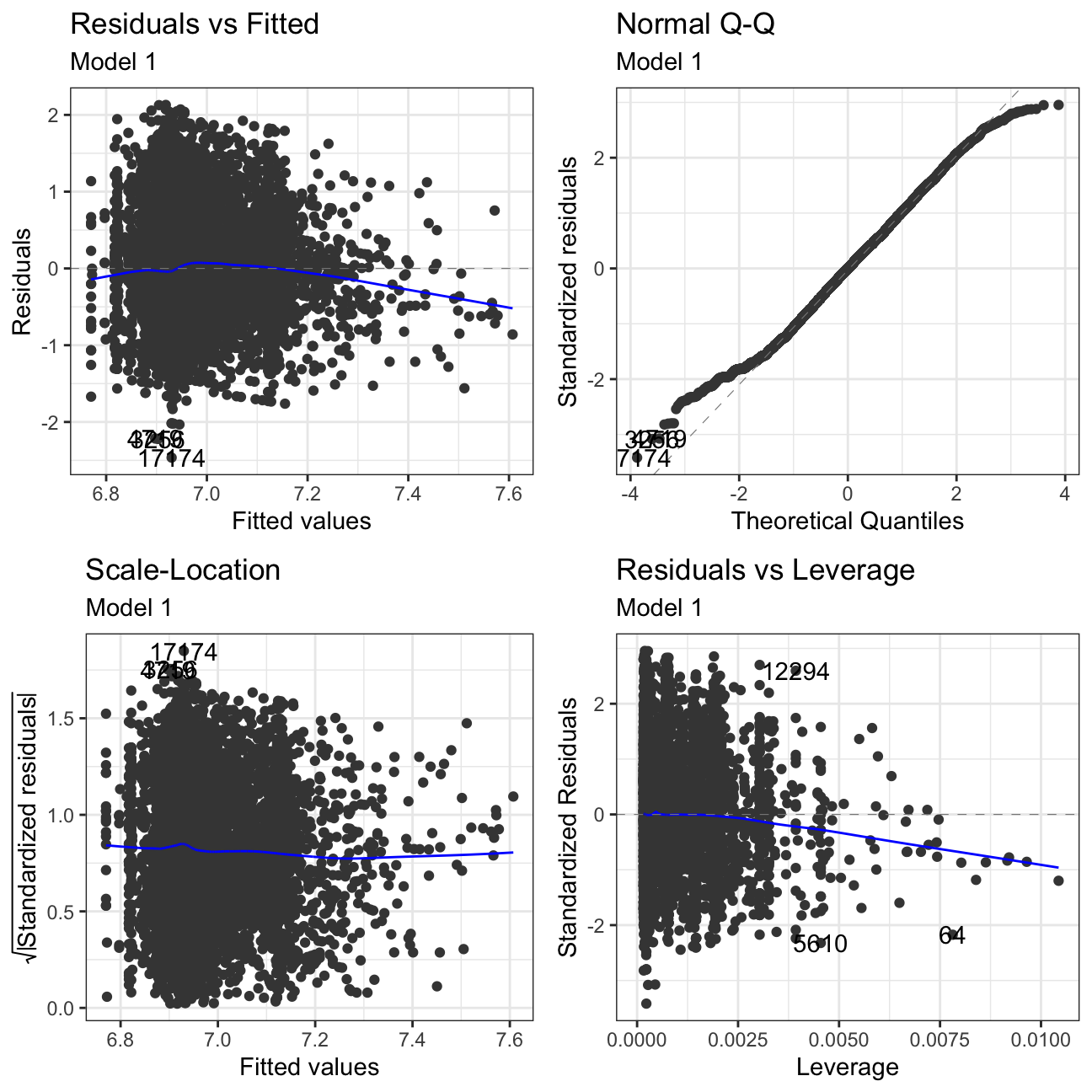
#Using autoplot to check residuals of our regression model
ggfortify:::autoplot.lm(model2) +
  labs(subtitle = "Model 2") +
  theme_bw()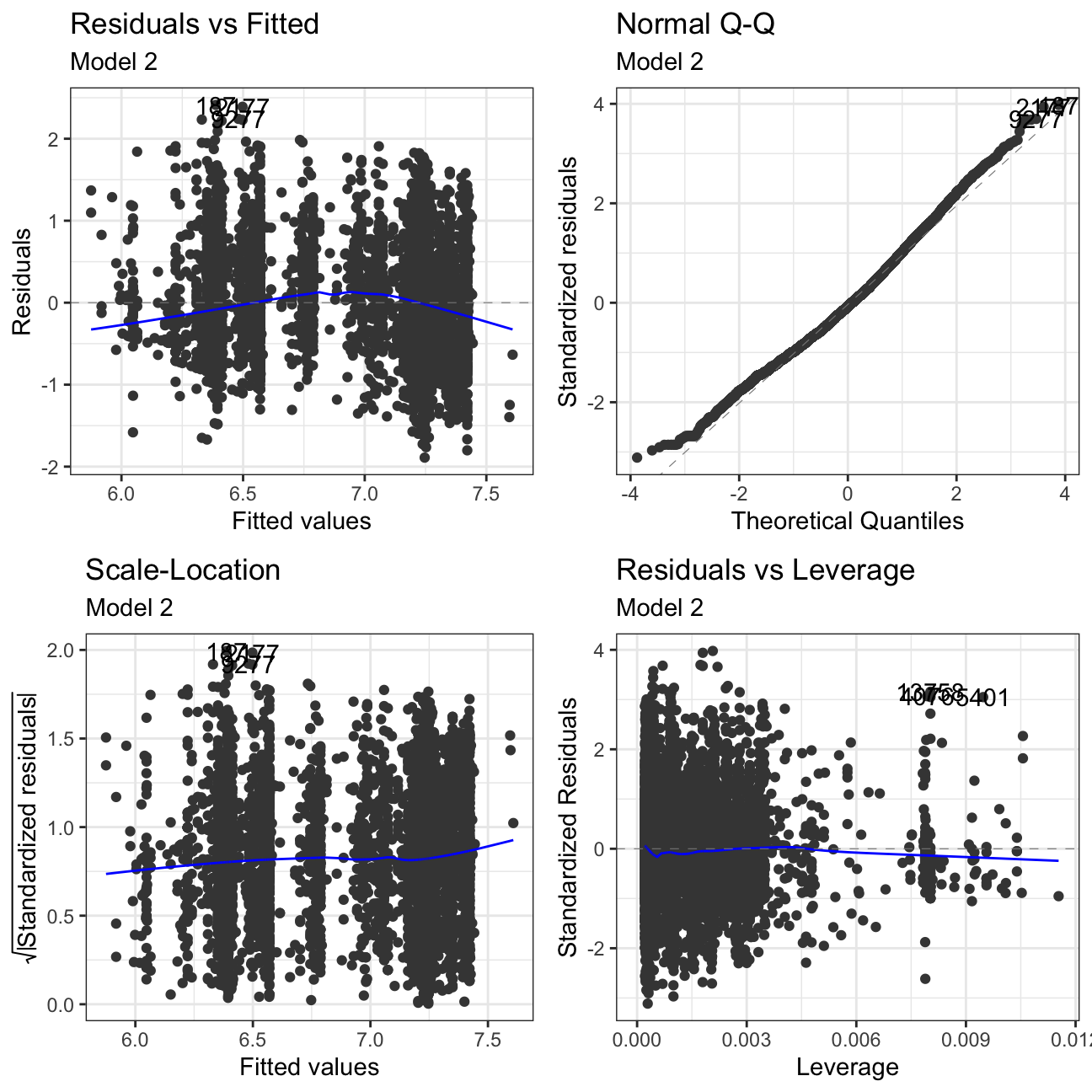
#Using autoplot to check residuals of our regression model
ggfortify:::autoplot.lm(model3) +
  labs(subtitle = "Model 3") +
  theme_bw()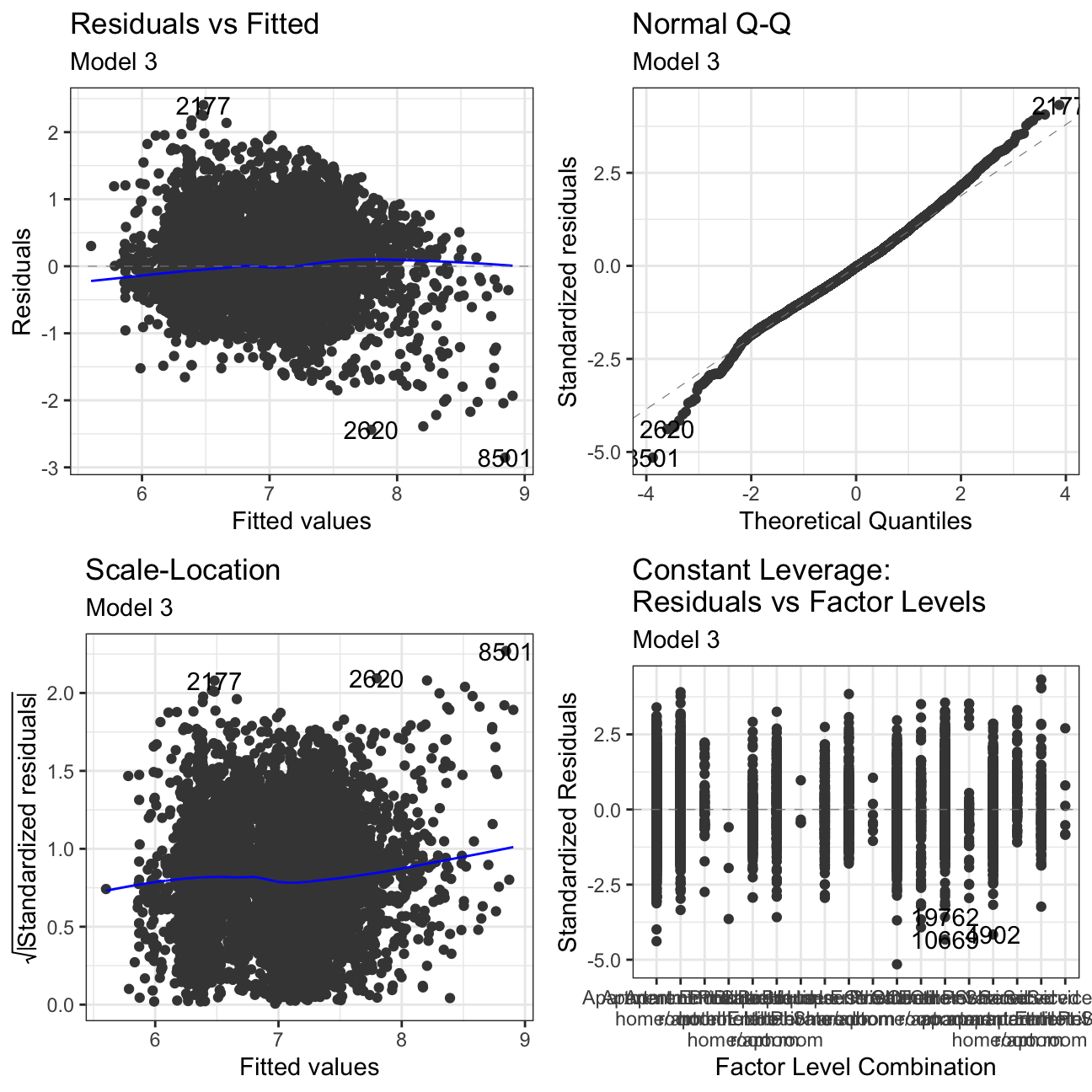
#Using autoplot to check residuals of our regression model
ggfortify:::autoplot.lm(model4) +
  labs(subtitle = "Model 4") +
  theme_bw()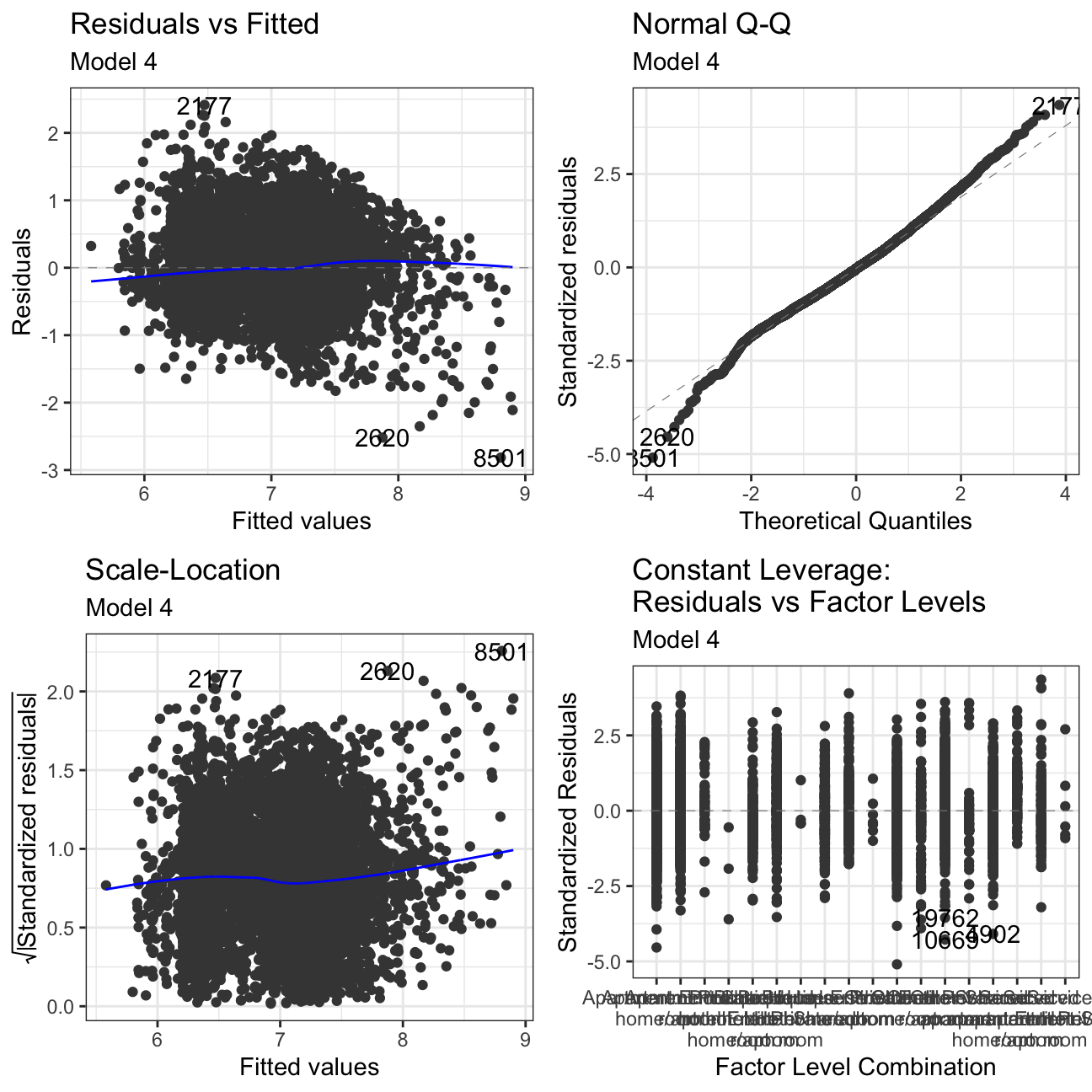
#Using autoplot to check residuals of our regression model
ggfortify:::autoplot.lm(model5) +
  labs(subtitle = "Model 5") +
  theme_bw()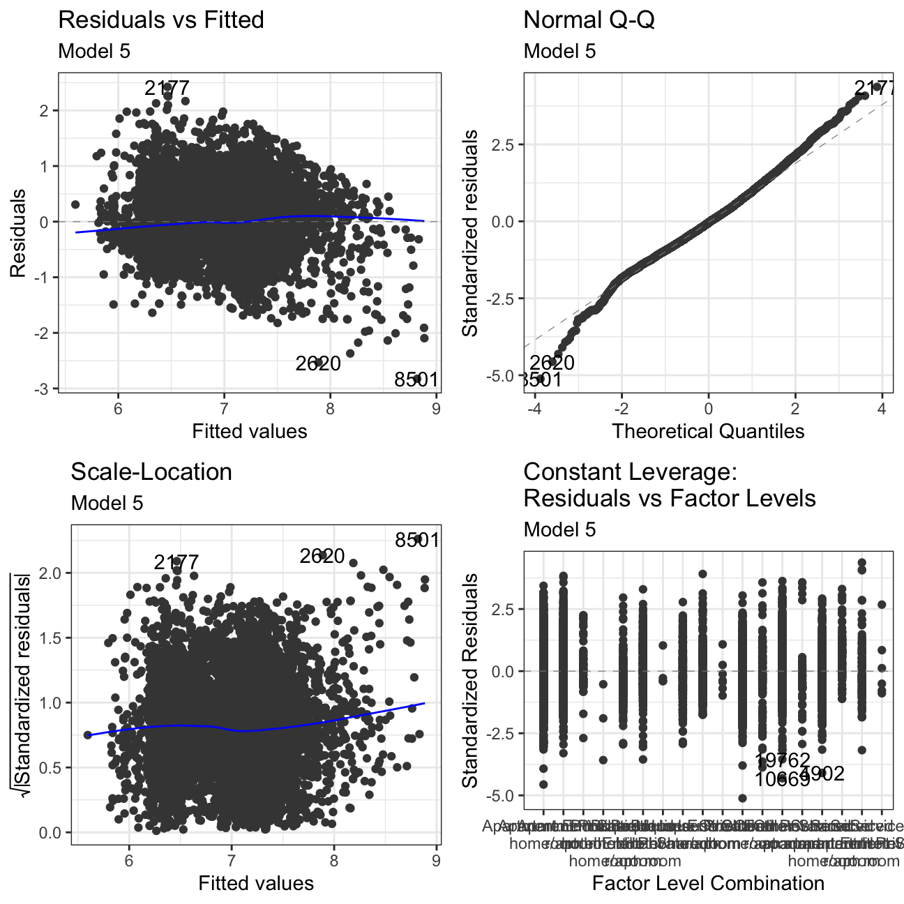
#Using autoplot to check residuals of our regression model
ggfortify:::autoplot.lm(model6) +
  labs(subtitle = "Model 6") +
  theme_bw()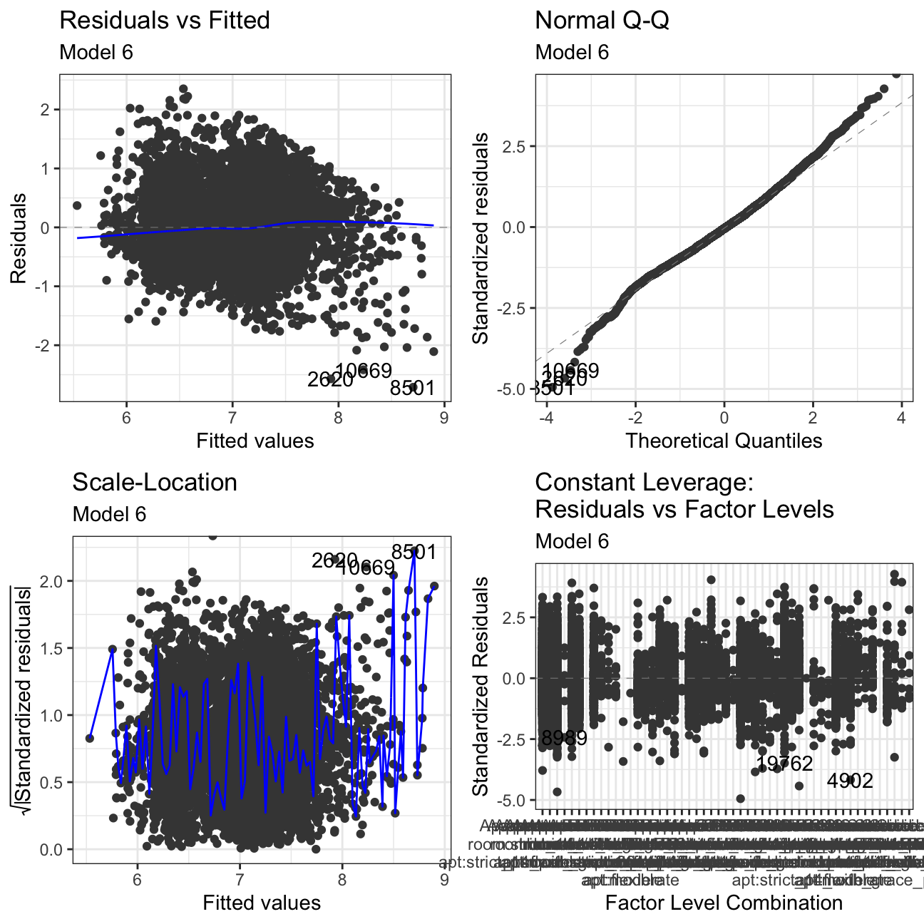
#Using autoplot to check residuals of our regression model
ggfortify:::autoplot.lm(model7) +
  labs(subtitle = "Model 7") +
  theme_bw()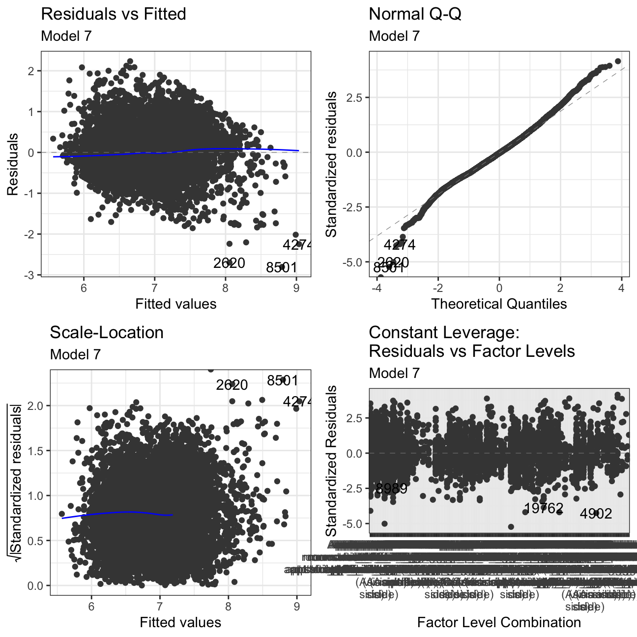
Residuals vs Fitted: There is no clear pattern in the plot. If we had pattern, it would mean that the data have a linear relationship, which was not defined by the model and was omitted out in the residuals.
Normal Q-Q: The Normal Q-Q Plot only has a limited S form. If we cut off more outliers, we would get a straighter line. The S shape means that we have extremer values at the tails - meaning we have very low/very high prices for there given characteristics.
Scale-Location: This plot shows if residuals are spread equally along with the ranges of predictors. This is how one can check the assumption of equal variance. It’s acceptable if you see a horizontal line with equally spread points. Our Data set looks like the residuals are spread randomly.
Residuals vs Leverage: This plot helps us to find influential cases if any, as not all outliers are influential in linear regression. In our models, there are no influential cases, as we can’t see Cook’s distance lines (a red dashed line) because all cases are well inside of the Cook’s distance lines.
Summary of the models developed
During the development of our models, we have been assessing the improvements and the value of our changes looking at the p-values and adjusted R-squared, leading to the conclusion that our last model (model7) has the best predictive capacity. However, let us recap all the models that we have developed so far and compare the improvements between them. We will do this using huxtable.
# Produce summary table comparing models using huxtable::huxreg()
huxtable::huxreg(model1, model2, model3, model4, model5, model6, model7,
       statistics = c('#observations' = 'nobs',
                      'R squared' = 'r.squared',
                      'Adj. R Squared' = 'adj.r.squared',
                      'Residual SE' = 'sigma'),
       bold_signif = 0.05,
       stars = NULL
)| (1) | (2) | (3) | (4) | (5) | (6) | (7) | |
|---|---|---|---|---|---|---|---|
| (Intercept) | 6.793 | 7.031 | 6.492 | 6.529 | 6.519 | 6.474 | 6.535 |
| (0.050) | (0.042) | (0.042) | (0.042) | (0.042) | (0.042) | (0.042) | |
| prop_type_simplifiedBoutique hotel | 0.010 | 0.392 | 0.348 | 0.352 | 0.348 | 0.347 | 0.308 |
| (0.033) | (0.031) | (0.029) | (0.029) | (0.029) | (0.029) | (0.028) | |
| prop_type_simplifiedHouse | -0.052 | 0.017 | -0.008 | -0.010 | -0.009 | -0.002 | 0.022 |
| (0.033) | (0.027) | (0.025) | (0.025) | (0.025) | (0.025) | (0.025) | |
| prop_type_simplifiedOther | -0.005 | 0.175 | 0.142 | 0.143 | 0.142 | 0.146 | 0.143 |
| (0.021) | (0.019) | (0.017) | (0.017) | (0.017) | (0.017) | (0.017) | |
| prop_type_simplifiedServiced apartment | 0.192 | 0.103 | 0.092 | 0.104 | 0.102 | 0.106 | 0.107 |
| (0.028) | (0.024) | (0.022) | (0.022) | (0.022) | (0.022) | (0.022) | |
| number_of_reviews | 0.002 | 0.000 | 0.000 | -0.000 | -0.000 | -0.000 | 0.001 |
| (0.000) | (0.000) | (0.000) | (0.000) | (0.000) | (0.000) | (0.000) | |
| review_scores_rating | 0.001 | 0.002 | 0.003 | 0.002 | 0.002 | 0.002 | 0.003 |
| (0.001) | (0.000) | (0.000) | (0.000) | (0.000) | (0.000) | (0.000) | |
| room_typeHotel room | -0.363 | -0.198 | -0.186 | -0.188 | -0.184 | -0.209 | |
| (0.032) | (0.030) | (0.030) | (0.030) | (0.030) | (0.029) | ||
| room_typePrivate room | -0.851 | -0.604 | -0.597 | -0.596 | -0.579 | -0.580 | |
| (0.014) | (0.014) | (0.014) | (0.014) | (0.014) | (0.014) | ||
| room_typeShared room | -1.199 | -1.001 | -0.999 | -0.998 | -0.984 | -1.005 | |
| (0.054) | (0.050) | (0.050) | (0.050) | (0.050) | (0.049) | ||
| bathrooms | -0.043 | -0.044 | -0.044 | -0.047 | -0.048 | ||
| (0.010) | (0.010) | (0.010) | (0.009) | (0.009) | |||
| bedrooms | 0.039 | 0.040 | 0.041 | 0.043 | 0.049 | ||
| (0.008) | (0.008) | (0.008) | (0.008) | (0.008) | |||
| beds | -0.004 | -0.004 | -0.004 | -0.004 | -0.007 | ||
| (0.004) | (0.004) | (0.004) | (0.004) | (0.004) | |||
| accommodates | 0.122 | 0.121 | 0.121 | 0.118 | 0.117 | ||
| (0.004) | (0.004) | (0.004) | (0.004) | (0.004) | |||
| host_is_superhostTRUE | 0.109 | 0.107 | 0.095 | 0.126 | |||
| (0.015) | (0.015) | (0.015) | (0.015) | ||||
| is_location_exactTRUE | 0.025 | 0.021 | 0.014 | ||||
| (0.012) | (0.012) | (0.012) | |||||
| cancellation_policymoderate | 0.115 | 0.110 | |||||
| (0.014) | (0.014) | ||||||
| cancellation_policystrict | 0.423 | 0.310 | |||||
| (0.551) | (0.539) | ||||||
| cancellation_policystrict_14_with_grace_period | 0.136 | 0.122 | |||||
| (0.014) | (0.014) | ||||||
| cancellation_policysuper_strict_30 | 1.004 | 0.916 | |||||
| (0.184) | (0.180) | ||||||
| cancellation_policysuper_strict_60 | 1.283 | 1.310 | |||||
| (0.551) | (0.540) | ||||||
| neighbourhood_simplifiedEast (Asian side) | -0.236 | ||||||
| (0.016) | |||||||
| neighbourhood_simplifiedNorth | -0.089 | ||||||
| (0.044) | |||||||
| neighbourhood_simplifiedOutskirt | -0.144 | ||||||
| (0.028) | |||||||
| neighbourhood_simplifiedWest | -0.284 | ||||||
| (0.023) | |||||||
| reviews_per_month | -0.094 | ||||||
| (0.009) | |||||||
| #observations | 9522 | 9522 | 9423 | 9423 | 9423 | 9423 | 9422 |
| R squared | 0.014 | 0.301 | 0.411 | 0.414 | 0.414 | 0.423 | 0.449 |
| Adj. R Squared | 0.013 | 0.301 | 0.410 | 0.413 | 0.413 | 0.422 | 0.447 |
| Residual SE | 0.721 | 0.607 | 0.557 | 0.555 | 0.555 | 0.551 | 0.539 |
Prediction
Finally, it is the moment to use our best model (model7) for prediction. We will use it to predict the total cost to stay at an Airbnb for four nights. The prediction will be made for an apartment with a private room, have at least ten reviews, and an average rating of at least 90. As we are looking for an Airbnb for tourist, we make the assumption that the tourist wants to live in the city centre. Additionally, we make the assumption that we need two bedrooms and one shared bathroom. The appropriate 95% confidence interval will be included, and both the point prediction and interval will be reported in terms of price_4_nights. As we used a log(price_4_nights) model, we will use anti-log to convert the value in $.
# Adjust the data set to the specifications of our prediction (the type of property whose price we want to predict)

prediction_Istanbul <- listing_price %>%

        filter(room_type == "Private room",
        number_of_reviews >= 10,
        review_scores_rating >= 90,
        prop_type_simplified == "Apartment",
        bathrooms == 1,
        bedrooms == 2,
        beds == 2,
        accommodates == 2,
        is_location_exact = TRUE,
        cancellation_policy == "flexible",
        neighbourhood_simplified == c("Centre"))

#Anti-log price by calculatin its exponential value, because exp(ln(x)) = x

model_predictions_log <- exp(predict(model7, newdata = prediction_Istanbul, interval = "confidence"))


paste("The predicted price for two people to stay four nights in Istanbul is $", round( model_predictions_log [1], 2), "with a 95% confidence interval between $", round(model_predictions_log[2], 2), "and $", round(model_predictions_log[3],2))
## [1] "The predicted price for two people to stay four nights in Istanbul is $ 670.8 with a 95% confidence interval between $ 644.74 and $ 697.92"